채린's datascience

Let’s start with an example: Suppose you're given a dataset that contains the size (in terms of area) of different houses and their market price. Your goal is to come up with an algorithm that will take the size of the house as its input and return its market price as the output.

In this example, the input variable i.e the size of the house, is called the independent variable (X), the output variable i.e house price is called the dependent variable (Y), and this algorithm is an example of supervised learning. 

In supervised learning, algorithms are trained using "labeled" data (in this example, the dependent variable - house price, is considered a label for each house), and trained on that basis, the algorithm can predict an output for instances where this label (house price) is not known. "Labeled data" in this context simply means that the data is already tagged with the correct output. So in the above example, we already know the correct market price for each house, and that data is used to teach the algorithm so that it can correctly predict the house price for any future house for which the price may not be known.

The reason this paradigm of machine learning is known as supervised learning, is because it is similar to the process of supervision that a teacher would conduct on the test results of a student on an examination, for example. The answers the student gives (predictions) are evaluated against the correct answers (the labels) that the teacher knows for those questions, and the difference (error) is what the student would need to minimize to score perfectly on the exam. This is exactly how machine learning algorithms of this category learn, and that is why the class of techniques is known as supervised learning.

There are mainly 2 types of supervised learning algorithms:

1. Regression, where your output variable is a continuous variable, for example, the price of a house.
2. Classification, where your output variable is categorical, for example, approve the loan or not i.e. yes or no categories.

In this lecture, we will be learning about regression algorithms, which obviously find great use in the machine learning prediction of several numerical variables we would be interested in estimating, such as price, income, age, etc.

Linear Regression

Linear Regression is useful for finding the linear relationship between the independent and dependent variables of a dataset. In the previous example, the independent variable was the size of the house and the dependent variable its market price.

This relationship is given by the linear equation: 

Where 

 is the constant term in the equation, 

 is the coefficient of the variable 

, 

is the difference between the actual value 

 and the predicted value (

).

 and 

 are called the parameters of the linear equation, while 

 and 

 are the independent and dependent variables respectively.

What is an error?

With given 

 and 

 in the training data, the aim is to estimate 

 and 

 in such a way that the given equation fits the training data the best. The difference between the actual value and the predicted value is called the error or residual. Mathematically, it can be given as follows:

In order to estimate the best fit line, we need to estimate the values of 

 and 

  which requires minimizing the mean squared error. To calculate the mean squared error, we add the square of each error term and divide the sum with the total number of records: 

The equation of that best fit line can be given as follows: 

Where 

 is the predicted value, 

 are the estimated parameters.

This equation is called the linear regression model. The above explanation is demonstrated in the below picture:

Before applying the model over unseen data, it is important to check its performance to make it reliable. There are a few metrics to measure the performance of a regression model.

1. R-squared: R-squared is a useful performance metric to understand how well the regression model has fitted over the training data. For example, an R-squared of 80% reveals that 80% of the training data fit the regression model. A higher R-squared value generally indicates a better fit for the model.
   
   
2. Adjusted R-squared: The adjusted R-squared is a modified version of R-squared that takes into account the number of independent variables present in the model. When a new variable is added, adjusted R-squared increases if that variable adds value to the model, and decreases if it does not. Hence, adjusted R-squared is a better choice of metric than R-squared to evaluate the quality of a regression model with multiple independent variables, because adjusted R-squared only remains high when all those independent variables are required to predict the value of the dependent variable well; it decreases if there are any independent variables which don't have a significant effect on the predicted variable.
   
   
3. RMSE: RMSE stands for Root Mean Squared Error. It is calculated as the square root of the mean of the squared differences between actual outputs and predictions. The lower the RMSE the better the performance of the model. 
   Mathematically it can be given as follows:     
            

   

1. Accuracy란?

전체 샘플 개수 중에 나의 알고리즘이 예측한 개수를 나타냅니다. 

예를 들어, Accuracy가 80인 경우 100개중 80개의 정답을 맞춘 것 입니다. 

여기서 중요한 것은 무조건 balanced data의 경우에만 이 지표를 사용하는 것이 맞습니다. 

예를 들어, 암환자는 1명, 암환자가 아닌 사람은 999명인 상황에서 우리가 만든 모델이 

'암환자가 아닌 환자로 모두 판별하는 모델'로 만들어 졌다면, 

Accuracy는 전체 1000명중 999명을 암환자가 아닌것으로 판단하였기 때문에 99%의 Accuracy값을 갖게됩니다. 

이말은, 쉽게 말해 암환자가 아니라고만 말하고 찍어도 99프로 이상의 정답률을 낸다는 것입니다. 

2. Precision과 Recall, 둘의 조화평균 F1-score

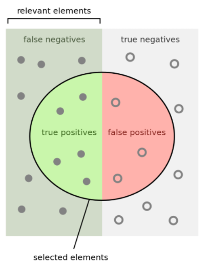
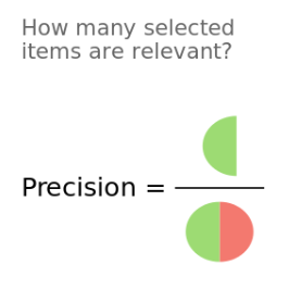
Precision(정밀도)는 PPV(Positive Positive Value)와 같은 의미를 가진 용어입니다.

의미를 살펴본다면, 내 알고리즘이 Positive(양성)이라고 예측한 것 들중에 실제로 Positive인 것들이 몇개나 되는지를 나타냅니다. 

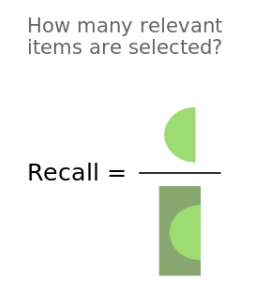
Recall(재현율)은 Sensitivity(민감도)와 같은 의미를 가진 용어입니다. 

실제 Positive인 데이터들 중 내 알고리즘이 Positive라고 예측한 것이 몇개나 되는지를 나타냅니다. 

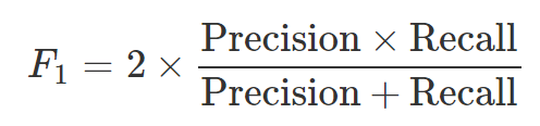
F1-score는 Precision과 Recall을 모두 고려하고 싶을때 사용하는 지표로 약간씩 다른 관점에서 Positive를 얼마나 잘 예측하는지 성능평가하는 값입니다. 

보통은, ROC커브를 그려 AUC로 성능을 평가하지만, Precision과 Recall을 이용한 경우는 Precision-Recall Curve를 그려서 확인합니다. 

3. Precision-Recall Curve

Threshold에 따라, Precision과 Recall은 trade-off관계를 가지며 threshold에 의한 함수라는것을 알 수 있습니다. 

Threshold를 조정하여 Precision-Recall Plot을 그리는 것을 설명해놓은 좋은 블로그를 공유해 놓습니다. 

https://ardentdays.tistory.com/20

https://rk1993.tistory.com/entry/Ridge-regression%EC%99%80-Lasso-regression-%EC%89%BD%EA%B2%8C-%EC%9D%B4%ED%95%B4%ED%95%98%EA%B8%B0

• Sensitivity(민감도): 질병이 있는 사람을 양성으로 검출하는 능력
• Specificity(특이도): 질병이 없는 사람을 음성으로 검출하는 능력
• Positive Predictive Value(양성예측치): 양성으로 나온 것 중에 실제로 질병이 있을 확률
• Negative Predictive Value(음성 예측치): 음성으로 나온 것 중에 실제로 질병이 없을 확률

3months.tistory.com/318

참고하기 좋은 블로그

abundant class(주로 정상데이터)와 rare class(이상데이터 그룹)의 비율이 1:99와 같이 극단적인 경우가 발생하는 경우, 

크게 두가지 방법으로 모델의 잘못된 판단을 막을 수 있습니다. 

1. sampling을 하는 것

2. 모델의 cost를 주어 모델 내에서 개선하는 방법

이번 포스팅에서는 sampling중 down-sampling과 up-sampling의 방법론들을 다룰 것 입니다.

1. Down-sampling

Under-sampling의 장점은 필요없는 데이터를 지우기 때문에, 계산시간이 빠르지만 단점은 지워진 데이터들로 인해 정보손실이 발생할 수 있습니다. 

• random down-sampling: 랜덤하게 abundant class의 instance를 추출해서 rare class와 1:1 비율을 맞춘 데이터 셋으로 학습시킵니다. 매번 랜덤하게 샘플링되기 때문에 경계선이 달라져 결과가 달리나오지만 꽤나 좋은 모델로 평가받고 있습니다. 
• Tomek links down-sampling: Tomek-links라는 것은 abundant class의 instance와 rare class의 instance를 2차원 평면에 뿌렸을 때, 둘 사이를 직선으로 열결했을때 이를 방해하는 다른 instance가 없을 경우에 그 직선을 말합니다. 이때, Tomek-links에 연결된 정상데이터들을 지움으로써 분류경계선을 새로 그을 수 있게 됩니다. 

•  CNN(Condensed Nearest Neighbor) : 1-NN를 사용해서 abundant와 rare사이의 1개의 관측치를 골라서 어떤 그룹에 더 가까운지 판단하여 가까운 그룹에 데이터로 속하게 함. 만약, rare class에 가깝다면 abundant class의 instance를 rare로 변경하고, 나머지 abundant class data를 모두 지웁니다. 그 후, rare class로 분류되었던 abundant class의 data를 다시 abundant class로 변경해줍니다. 이때, 사용하는 NN은 k-NN이 아닌 무조건 1-NN을 사용해야합니다. 

• OSS: Tomet-links에서 나온 under-sampling 데이터와, CNN에서 나온 under-sampling데이터를 합치는 것입니다. OSS

2. Over-sampling

단점: 소수클래스에 과적합이 생길 수 있습니다. 

• Resampling: rare class의 instance를 랜덤복원추출하여 데이터를 증가시키는 방법입니다. 
• SMOTE (Sythetic Minority Oversampling technique): resampling 했을때 over-fitting되는 문제를 해결하기 위해 나온 방법론으로 up-sampling에서 주로 사용되는 방법입니다.  
• Boarderline SMOTE: 경계부분에서 over-sampling을 하는 방법입니다. 이상데이터와 정상데이터 사이의 데이터들 위주로 증폭시키기 위한 방법입니다. 사실, 전체 정상데이터와 이상데이터 사이에 SMOTE를 사용하면, 경계선 주변부에 데이터들이 생성되는것이외에 이상데이터 바깥쪽에도 데이터가 생성될 가능성이 높습니다. 하지만, 이런 데이터들은 모델을 학습시키기에 좋은 데이터들은 아니기 때문에 경계선 주위에 데이터를 생성할 수 있도록, 경계선 주위의 정상데이터들로 SMOTE샘플링을 하는 방법입니다. 

여기서?

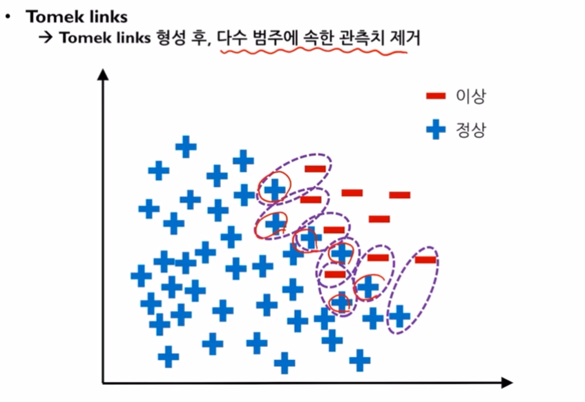
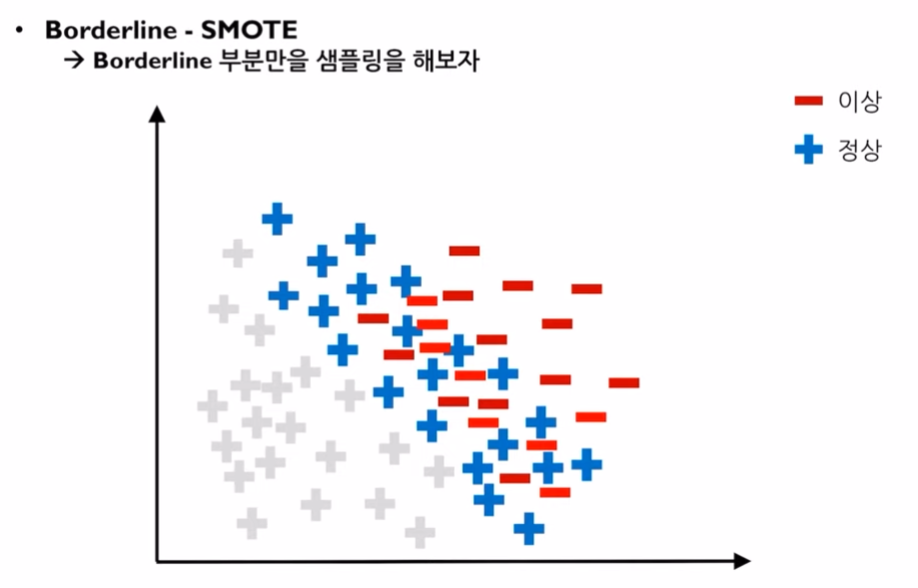
컴퓨터가 Boarderline을 판단하는 방법은, k를 정해 그룹핑을 하여 k개의 데이터가 모두 소수 관측치라면 이를 'safe 관측치'라고 부릅니다. 그리고 이것은 boarderline이 될 수 없습니다. 

하지만, 다른 k개의 그룹을 했을때, 다수 관측치가 k/2이상이라면 이를 boarderline이라고 하며 'danger 관측치'라고 부릅니다. k개의 그룹에서 다수의 데이터가 또 너무 많이 존재할 경우 이를 'noise 관측치'라고 합니다.

따라서, Boarderline SMOTE sampling의 경우에는 danger 관측치에서 SMOTE sampling을 하는것을 말합니다. 

• ADASYN(Adaptive Synthetic sampling approach): 

<인공지능공학소의 김성범 소장님의 강의를 참고하여 작성합니다. >

python 비대칭 데이터 문제 해결:

datascienceschool.net/03%20machine%20learning/14.02%20%EB%B9%84%EB%8C%80%EC%B9%AD%20%EB%8D%B0%EC%9D%B4%ED%84%B0%20%EB%AC%B8%EC%A0%9C.html

• up-sampling을 할때 이점과 영향
• SMOTE 알고리즘

1.  up-sampling을 할때 이점과 영향

down-sampling은 데이터 수가 많다고 생각될 경우 사용을 하지만, 보통 데이터수가 많으면 많을수록 좋기때문에 

up-sampling을 down-sampling보다 선호합니다.

unsupervised machine learning model과 다르게 supervised model은 outcome의 확률분포를 학습하지 않습니다. 

따라서, training data의 outcome비율을 1:1로 맞추기 위해 up-sampling을 해주어도 절대! test data의 outcome 비율을 변경하기 위해 test data도 up-sampling을 해주지 않습니다!

'데이터의 비율을 달리하여 학습한 모델인데 test data도 비슷한 분포를 띄어야 학습결과가 좋게 나온다?'라고 쉽게 오해할 수 있습니다.

하지만, 기본적으로 test data는 변경하여 사용하는 것이 아닐 뿐더러

1) 모델이 학습할 때, supervised model의 경우 outocme의 비율을 학습하지 않습니다. 

upsampling의 목적은 imbalance한 데이터를 학습할 경우 모델이 한쪽 class로 판단하는 모델로 빠르게 도달하지 않도록 방해하는 역할을 합니다. up-sampling은 rare class의 데이터들을 복원추출하여 데이터를 늘리는것이기 때문에 다량의 학습데이터를 학습하는 효과를 주는것이 아닌, rare class의 특성을 반영한 데이터들이 늘어나서 over-fitting이 됩니다. 

2) test data의 분포를 모델이 체크하지 않습니다.

training data로 모델을 만들고 나서 test data를 이용해 모델의 성능을 평가하는데 이때, test data는 한개씩 들어가서 이를 (binary의 경우) 1,0중에 판단하여 결과값만 내기때문에 outcome의 분포는 상관하지 않습니다.  

2. SMOTE 알고리즘

Up-sampling의 하나의 종류로, k 최근접 이웃 method를 이용한 방법입니다.

우선, k 최근접 이웃 모델을 사용할때처럼 rare class의 데이터들중 하나의 데이터를 선택하고 그 주변에 얼마나 많은 k개의 이웃을 선택할 것인지 정해줍니다. 

예를 들어, k가 5개이면, 정해진 중심으로부터 5개의 이웃만 고려를 할것입니다.

그리고 간단히, SMOTE알고리즘이 구동되는 방식을 보자면,

X는 선택한 점, X(nn)은 그 주변에 선택된 하나의 근접이웃, u는 균등분포입니다. 

예를 들면, X가 (5,1)이고 X(nn)이 (2,3)인 경우 X(nn)부터 X까지의 거리를 표현하면 (-3,2)가 됩니다. 

두 점사이 거리에서 0부터 1사이의 값이 랜덤으로 곱해져서 둘 사이에 위치하는 새로운 데이터가 생성이 될 것입니다. 

이 방법은 rare class의 있는 데이터를 고르는것이 아닌, 비슷한 데이터를 생성해내기 때문에 약간의 차이는 있지만 

그래도 over-fitting의 문제를 고려해야합니다. 

reference: www.youtube.com/watch?v=Vhwz228VrIk

• GAN이란?
• GAN의 학습방법

포스팅 목적: 의학도나 방사선사들의 훈련에는 많은 영상이 필요하나, 구조적 법적 문제로 대량의 영상을 공유하기가 쉽지 않습니다. 데이터의 양이 적어 해결되지 않는 문제들을 개선하고자 공부하였고 이 내용을 포스팅합니다. 

reference: 

논문: Towards generative adversarial networks as a new paradigm for radiology education

참고 영상: 

tv.naver.com/v/1947034

1. GAN이란?

GAN(Generative Adversarial Network)로 적대적 생성 모델이라고 합니다. 

하나씩 뜯어서 보자면, 생성모델이라는 관점에서 

머신러닝에서 만들어내는 예측 결과나, continuous variable의 interval prediction값이 아닌(가장 높은 확률 혹은 likelihood를 찾아내는 행위), 데이터의 형태를 만들어내는 모델입니다. 

데이터의 형태는 분포 혹은 분산을 의미하고 데이터의 형태를 만들어 낸다는 것은 '실제적인 형태'를 갖춘 데이터를 만든다는 뜻입니다.  

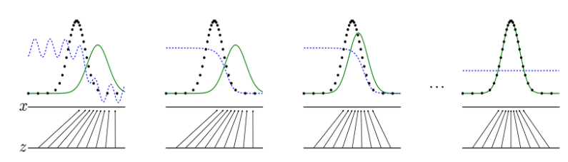
위 그림에서 보듯이, 기존에 분포를 학습해서 데이터의 형태를 찾아나가고 이를 만들어 내는 것입니다. 

또한, 적대적 생성의 의미 측면에서는,

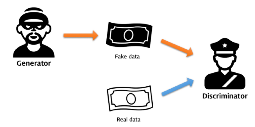
GAN의 핵심 아이디어로, 각각의 역할을 가진 두개의 모델로 진짜같은 가짜를 생성해주는 능력을 키워주는 것을 의미합니다. 

예를 들어, 위조범이 가짜 지폐를 만들어내고, 경찰은 가짜지폐를 찾아내는 역할을 합니다. 더욱 더 서로가 위조지폐를 정교하게 만들고, 만들어진 위조지폐를 정확히 찾아내는 것으로 서로 적대적으로 능력을 키워주고 있습니다. 

이런 아이디어에서부터 '적대적'이라는 용어가 붙게 되었습니다. 

2. GAN의 학습방법

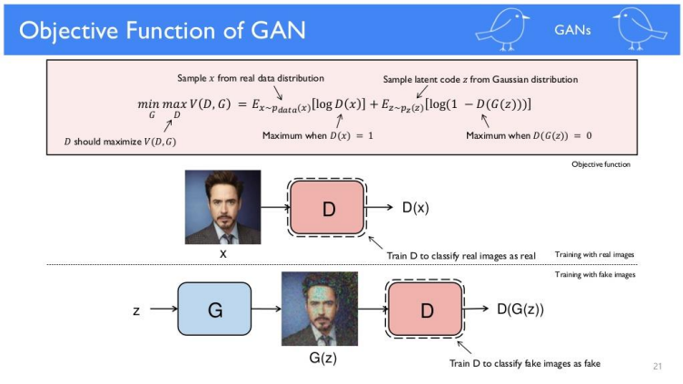
Discriminator는 CNN판별기처럼 네트워크 구성할 수 있습니다. Disciminator로 진짜 이미지는 1, 그렇지 않은 것은 0으로 학습을 시키고, z라는 랜덤백터를 넣어 Genarative학습을 시킨 이미지가 이미 학습된 D에 들어갔을때, 오로지 진짜 이미지로 판별할 수 있도록, G를 학습시키는 것입니다. 

G는 random한 noise를 생성해내는 vector z를 noise input으로 받고 D가 판별해내는 real image를 output으로 하는 neural network unit을 생성합니다. 

GAN의 코어 모델은 D와 G두개이고, mnist이미지를 real image로 D한테 '진짜'임을학습시키고, 

vector z와 G에 의해 생성된 Fake Image가 가짜라고 학습을 시켜 총 두번의 학습을 거칩니다. 

이때, 따로 학습되는 것이 아니라 1번의 과정에서 real image와 fake image를 D의 x input으로 합쳐서 학습합니다. 

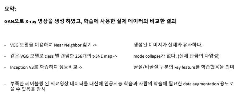
3. GAN을 이용해 영상 이미지를 만들고 AUC를 비교해보자. 

Real image만 사용했을때, AUC가 0.99정도 나왔고, 그 외에 GAN으로 만들어진 sample들로 학습했을때와, real과 gan을 적절히 섞어서 학습했을때 높은 AUC를 끌어낼 수 있었습니다. 

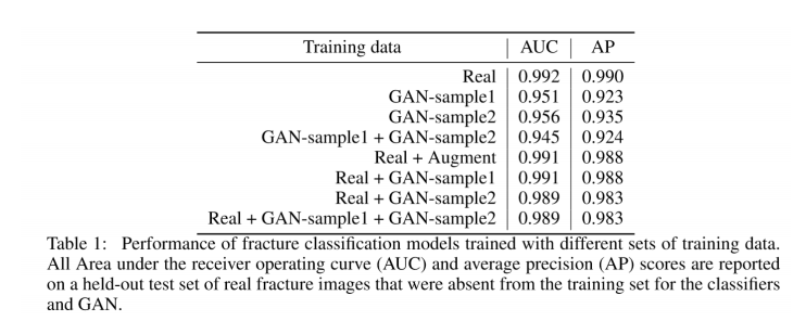
reference논문을 요약하자면,